20250209 모각코 활동 5회차

import pandas as pd  
import matplotlib.pyplot as plt  
  
from sklearn.model_selection import train_test_split  
from sklearn.preprocessing import StandardScaler  
from sklearn.linear_model import LogisticRegression  
  
from sklearn.tree import DecisionTreeClassifier  
from sklearn.tree import plot_tree

# 데이터 다운로드  
wine = pd.read_csv('https://bit.ly/wine_csv_data')

# 데이터 구조 확인  
print(wine.head())  # 처음 5개의 샘플  
print(wine.info())  # 데이터프레임의 각 열의 데이터 타입과 누락된 데이터 확인  
print(wine.describe())  # 통계 ( 평균, 표준편차, 최소, 최대, 중간값, 1사분위수, 3사분위수 )

# 판다스 데이터 프레임 -> 넘파이 배열  
data = wine[['alcohol', 'sugar', 'pH']].to_numpy()  
target = wine['class'].to_numpy()

# 데이터 나누기  
train_input, test_input, train_target, test_target = train_test_split(data, target, test_size=0.2, random_state=42)

# 나눈 데이터 형태 확인  
print(train_input.shape, test_input.shape)

# 데이터 전처리  
ss = StandardScaler()  
ss.fit(train_input)  
  
train_scaled = ss.transform(train_input)  
test_scaled = ss.transform(test_input)

lr = LogisticRegression()  
lr.fit(train_scaled, train_target)  
  
print(lr.score(train_scaled, train_target))  
print(lr.score(test_scaled, test_target))  
  
print(lr.coef_, lr.intercept_)  # 로지스틱 회귀가 학습한 계수와 절편

dt = DecisionTreeClassifier(random_state=42)  
dt.fit(train_scaled, train_target)  
  
print(dt.score(train_scaled, train_target))  
print(dt.score(test_scaled, test_target))

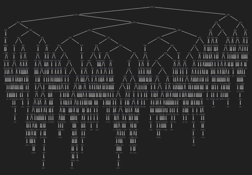
# 훈련 결과 시각화  
plt.figure(figsize=(10,7))  
plot_tree(dt)  
plt.show()

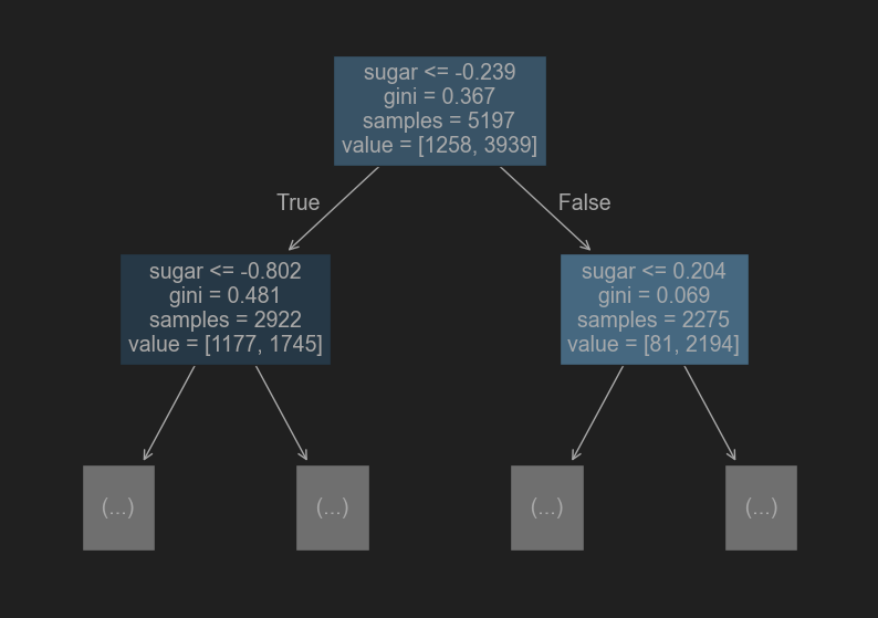
# 자세히 살펴보기  
plt.figure(figsize=(10,7))  
plot_tree(dt, max_depth=1, filled=True, feature_names=['alcohol', 'sugar', 'pH'])  
plt.show()

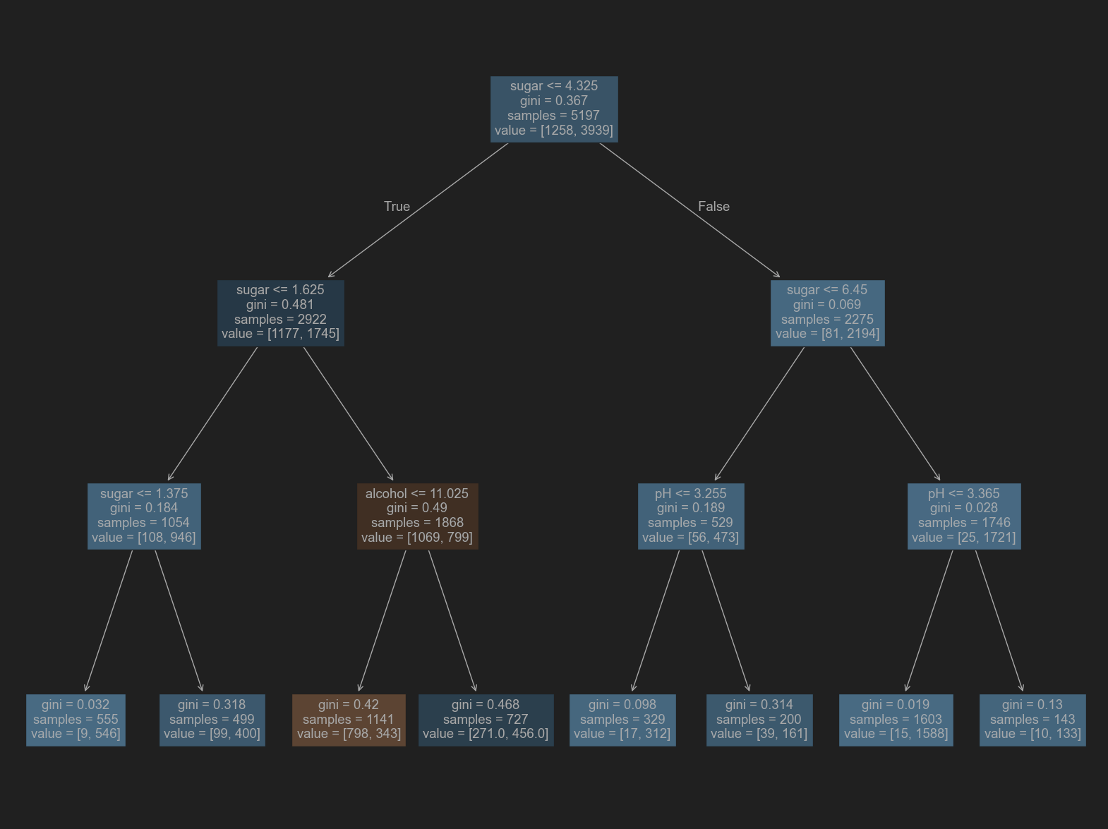
# 가지치기  
dt = DecisionTreeClassifier(max_depth=3, random_state=42)  
dt.fit(train_scaled, train_target)  
  
print(dt.score(train_scaled, train_target))  
print(dt.score(test_scaled, test_target))

# 가지치고 난 뒤의 훈련 시각화  
plt.figure(figsize=(20,15))  
plot_tree(dt, filled=True, feature_names=['alcohol', 'sugar', 'pH'])  
plt.show()

# 전처리 하기 전의 데이터들로 다시 훈련해보기  ->  결과는 같을 것.  
dt = DecisionTreeClassifier(max_depth=3, random_state=42)  
dt.fit(train_input, train_target)  
  
print(dt.score(train_input, train_target))  
print(dt.score(test_input, test_target))

# 시각화 -> 데이터를 전처리 하고 난 뒤에 훈련 한 것과 같은 트리를 갖지만, 특성값을 표준점수로 바꾸지 않았기 때문에 이해하기 더욱 쉬움.  
plt.figure(figsize=(20,15))  
plot_tree(dt, filled=True, feature_names=['alcohol', 'sugar', 'pH'])  
plt.show()

# 특성 중요도  
print(dt.feature_importances_)